Economic Resource Availability
Analysis of a community's ability to whether financial setbacks through social lending.
This project was completed as part of CS302 at UVM with Tom Nececkas and Mark Kirby. The following article is an overview of the project.
The Fed published a report where 40% of americans would have difficulty covering a $400 expense. Of those americans, 10% would borrow from a friend or family member to cover the expense. With an increasing number of people turning to crowdfunding sites such as GoFundMe 1, it is clear that people are becoming more reliant on the community to provide finanical relief. Our work develops a potential model for networks resources to insulate people in a community from financial setbacks.
Data
We used in income distribution from the Milwaukee Area Renters Study (MARS) which is publicly available here. The mean income is $1315.10 and median income is $1085.00. Approximately 13% report no income.
Details
We developed a model consisting of the following parameters:
- \(n\) nodes
- \(s\) proportion of savings
- \(a\) proportion of income that could be borrowed
- \(c\) expense
- \(I_k\) income of the kth individual
The goal was to determine the following using the MARS income distribution:
- Determine the relationship between the reduction of financial resources in a community and the number of connections for the community to become financially stable.
- Determine the relationship between each of the parameters and the number of connections.
A notion of “financial stability” is needed to find the relationships. An individual is considered financially stable if their expense \(c\) can be covered with their own resources or in addition to the resources of a close neighbor. Formally,
\[sI_k + \sum_{n\in\mathcal{N}_k}aI_n \ge c\]where \(\mathcal{N}_k\) is the neighborhood of the kth individual.
Assumptions
- Only an individual’s income is considered.
- Individuals can allocate resources to cover expenses.
- Homogeneity. Everyone experiences the same financial setback and willingness to lend their resources.
In addition, the edges are created randomly. In reality, social networks are often structured.
Procedure
Starting with \(n\) disjoint nodes, we randomly create edges until the condition for financial stability is met following a relative reduction in the total income \(p\in\{0.05i \mid 0 \le i \le 20\}\) and changing the parameters \(n\in\{20, 50, 100\}\), \(s\in\{0.1, 0.2, 0.4\}\), \(a\in\{0.1,0.2,0.4\}\), and \(c\in\{400, 800, 1600\}\). This is repeated for \(T=100\) trials.

Results


The trend between expense and number of edges is almost linear until it approaches the maximum possible number of edges. However, the scaling from each reduction in income is non-linearly increasing. It indicates the the growth in the number of edges per percentrage reduction in income exceeds linear growth.


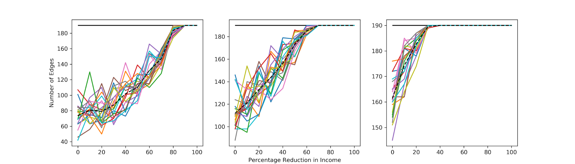
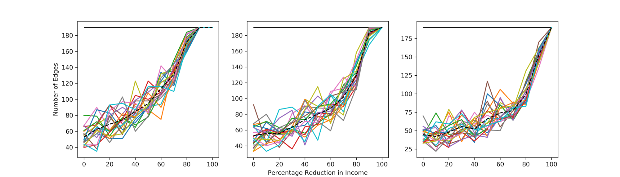
The trend between the number of edges with the number of people \(n\) in the community, increasing access \(a\) to resources, and expense \(c\) is as expected:
- More people in the network reduces the growth in the number of social connections to become financially stable.
- Fewer social connections are needed for individuals to become financially stable with greater community resources.
- Increasing costs increases the number of social connections. The common idea for 1 and 2 is increased community resources which reduces the growth in the number of edges. On the other hand, increasing costs is analogous to reducing the resources available in the community.
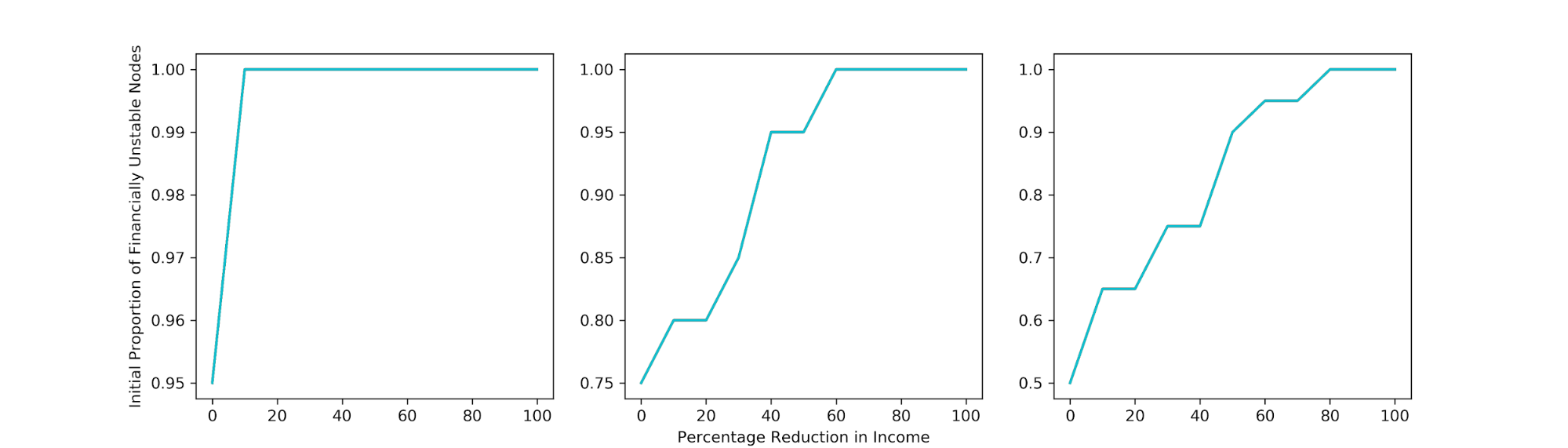
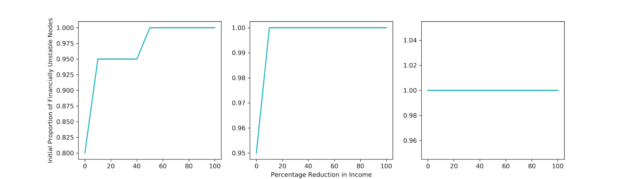
For savings, the results were unexpected. While increased savings reduced the initial proportion of those financially unstable, the number of social connections does not change significantly. It might be the case that those that require the most number of social connections are those with significantly low income.